Before an algorithm can be applied for sentiment classification, texts need to be vectorized. There are several different ways to do so - in this post, I try out TF-IDF.
TF-IDF
TF-IDF stands for “term frequency - inverse document frequency”. What it does is it counts how often a term \(t\) occurs in a given document \(d\) (\(\text{freq}_{t,d}\)), and weighs it against the occurrences of the same term \(t\) in the other documents of the corpus (\(\text{doc_freq}_{t}\)). Here, the documents are reviews. For example, stop words like “the” appear in every review, so the final weight of stop words is low. The opposite is true for a word like “rude”, which almost exclusively appears in reviews with negative sentiment.
The TF-IDF formula used by gensim is given by
\begin{align}
\text{tfidf}(t,d) = \text{freq}_{t,d} \cdot \log\big({\frac{N}{\text{doc_freq}_t}}\big)
\end{align}
To apply TF-IDF, a fixed vocabulary is necessary. This vocabulary is given by the gensim dictionary object which I have extracted in my last post. Every review will then be represented by a vector with a length equal to the vocabulary size. Every component of the vector represents a term in the vocabulary. The component value is calculated using the TF-IDF formula given above.
from gensim.models.phrases import Phrases, Phraser
from gensim.models import TfidfModel
from gensim.corpora import Dictionary
from gensim.matutils import corpus2csc

def apply_tfidf(dct: gensim.corpora.Dictionary, model: gensim.models.TfidfModel, df: pd.DataFrame, bigram: gensim.models.phrases.Phraser, trigram: gensim.models.phrases.Phraser) -> scipy.sparse.csc matrix:
    """
    Apply TF-IDF transformation
    Input:
    - dct: dictionary object
    - model: tfidf model
    - df: dataframe with column "text"
    - bigram: bigram phraser
    - trigram: trigram phraser
    """
    def wrapper_tfidf(generator):
        for item in generator:
            yield dct.doc2bow(trigram[bigram[item.text.split(" ")]])
    transformed_corpus = model[wrapper_tfidf(df.itertuples())]
    csc = corpus2csc(transformed_corpus,num_terms=len(dct)).transpose()
    return csc
Gensim’s TfidfModel does not directly return vectors, but objects of type gensim.interfaces.TransformedCorpus. Gensim offers a utility method which converts the object to a sparse scipy.sparse.csc_matrix. The sparse matrix can be fed to scikit-learn classifiers such as the logistic classifier. The reason why I did not directly use scikit-learn’s TfidfTransformer is because the dataset’s size causes it to run into a memory error.
Visualization
Now that I can vectorize the reviews, it would be interesting to visualize the different reviews.
Principal Component Analysis (PCA)
Given a centered dataset \(X \in \mathbb{R}^{N\times d}\), PCA constructs a set of \(k\lt d\) vectors \(u_1,\ldots,u_k \in \mathbb{R}^{d}\) which are orthonormal to each other and span a \(k\)-dimensional linear subspace. The dataset is approximated with these vectors as basis
\begin{align}
X \approx \sum_{i=1}^k X u_i \cdot u_i = XUU^T
\end{align}
where \(u_i\) is the \(i\)-th column of \(U\). The reconstruction error (sum of squared errors) is
\begin{align}
|| X-XUU^T ||_F^2 &= \text{tr}(X^T X) - \text{tr}(U^TX^TXU)
\end{align}
Minimizing the reconstruction error with respect to \(U\) is therefore equivalent to maximizing
\begin{align}
\text{tr}(U^T X^T X U) = \sum_i^k u_i^T X^T X u_i = \sum_i^k \text{Var}(Xu_i)
\end{align}
In other words, we try to find directions \(u_i\) along which the variance of the projection coordinate \(Xu_i\) (also called score) is maximal. It can be shown that choosing the \(k\) eigenvectors of \(X^T X\) with the largest eigenvalues is optimal. The score \(Xu_1\) of the eigenvector with the largest eigenvalue is called the first principal component, the score \(Xu_2\) the second principal component and so on.
One method to calculate the eigenvectors is through Singular Value Decomposition (SVD) of \(X\). Plugging in the SVD \(X = V_1 D V_2 ^T\) (\(V_1, V_2\) are orthonormal and \(D\) is a diagonal matrix) for the covariance matrix \(X^T X\) yields
\begin{align}
& X^T X = V_2 D V_1^T V_1 D V_2^T = V_2 D^2 V_2^T \newline
\iff & X^T X V_2 = V_2 D^2
\end{align}
The square of the singular values are therefore the eigenvalues and the columns of \(V_2\) are the eigenvectors.
Finally, the coordinates/scores \(XU\) with respect to the basis vectors in \(U\) can be used to visualize the data (for a 2-D plot \(U\) has only 2 columns).
t-Distributed Stochastic Neighbor Embedding (t-SNE)
In his Google Techtalk, the author of t-SNE shows several examples where PCA-based visualization fails to disentangle different classes. In these examples, PCA does a good job to preserve distances between points which are far apart, but doen’t pay much attention to the structure of the points close to each other. In contrast to PCA, t-SNE explicitly focuses on the local structure.
t-SNE introduces a similarity measure between points in the original dataset based on a Gaussian distribution
\begin{align}
p_{ij} = \frac{1}{2N} \cdot \Big(\frac{\exp{(-|x_i-x_j|/2\sigma_i^2)}}{\sum_{k\neq i}\exp(-|x_i-x_k|/2\sigma_i^2)} + \frac{\exp{(-|x_j-x_i|/2\sigma_j^2)}}{\sum_{k\neq j}\exp(-|x_j-x_k|/2\sigma_j^2)}\Big)
\end{align}
where \(\sigma_i\) is introduced in such a way that the density drops faster when there are more data points in the neighbourhood of \(x_i\).
In the lower dimensional dataset, another similarity measure is defined based on a student-t distribution with one degree of freedom:
\begin{align}
q_{ij} = \frac{(1+|y_i-y_j|^2)^{-1}}{\sum_k\sum_{l\neq k}(1+|y_k-y_l|^2)^{-1}}
\end{align}
Both \(p_{ij}\) and \(q_{ij}\) model joint distributions and these distributions shall be as similar as possible. The objective function becomes a minimization of the Kullback-Leibler divergence
\begin{align}
KL(p| q) = \sum_i\sum_{j\neq i} p_{ij} \log{\frac{p_{ij}}{q_{ij}}}
\end{align}
over the lower-dimensional representations \(y_1,\ldots,y_N\). For high \(p_{ij}\), \(q_{ij}\) needs to be high, too, to prevent the KL divergence from exploding. This is what preserves local structure. By choosing a student-t distribution in the target space, t-SNE also allows large distances to be exaggerated: The heavier tails of a t-distribution assigns a higher probability to points which have a large pairwise distance than a Gaussian distribution would. With this, similar data points can form clusters and the clusters in turn can be disentangled.
Application
I want to apply t-SNE to my data, but the dimensionality of the review vectors needs to reduced first to avoid performance issues. I use PCA to reduce the dimensionality of my data to 25 features before applying t-SNE.
X_csc = apply_tfidf(dct,model,X_resampled,bigram,trigram)
# use SVD only
reducer = TruncatedSVD(n_components=2)
X_reduced = reducer.fit_transform(X_csc)
points_svd=X_reduced
# use SVD for dimensionality reduction and then TSNE
reducer = TruncatedSVD(n_components=25)
X_reduced = reducer.fit_transform(X_csc)
tsne = TSNE(n_components=2, perplexity=100, learning_rate=250, n_iter=2500)
points_tsne = tsne.fit_transform(X_reduced)
fig = plt.figure()
ax1 = plt.subplot(121)
ax2 = plt.subplot(122)
colormap={-1:"r",0:"y",1:"g"}
colors=list(map(lambda x: colormap[x], y_resampled["sentiment"].tolist()))
ax1.scatter(points_svd[:,0],points_svd[:,1],s=5,c=colors)
ax2.scatter(points_tsne[:,0],points_tsne[:,1],s=5,c=colors)
plt.show()
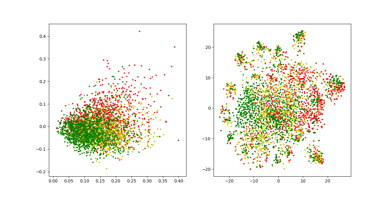
For the below visualizations, I used a subsample of my dataset which contains around 1,000 samples of each class. The right plot uses PCA directly for visualization. The left plot uses t-SNE on points with reduced dimensionality. There’s a considerable amount of overlap between the different sentiment classes in both visualizations. T-SNE disentangles the points, but not to the extent that it forms clear clusters for each class. It even seems to learn some local patterns that one would not expect, creating small, isolated islands containing samples of every class. The parameters I tried more or less yielded the same or worse results, but this doesn’t mean that there isn’t a parameter set that yields a better visualization.
Sentiment Classification
One of the main problems with this classification task is that the data set is heavily imbalanced. Training a logistic classifier naively with the given dataset will lead to a classifier that always predicts positive classes and still reaches an accuracy of at least 60%. To account for the imbalanced classes, I tried out two different approaches: class weighting and undersampling.
Scikit-learn’s LogisticRegression offers a parameter called class_weight. Setting it to “balanced” adjusts the class weights inversely proportional to class frequencies in the data. As a result, the final weights for the majority class will be smaller than without setting the parameter and the minority classes will have larger weights. To evaluate the trained model, I calculate precision and recall for all three classes. Below are the training results:
| |
Training Samples |
Test Samples |
| Positive |
3,161,079 |
790,282 |
| Negative |
1,072,732 |
268,329 |
| Neutral |
534,161 |
133,383 |
| |
Precision |
Recall |
| Positive |
0.9371339229458848 |
0.9146886807494033 |
| Negative |
0.8272568320165782 |
0.8569368200977159 |
| Neutral |
0.4726318297776906 |
0.5055891680349069 |
| Aggregated |
0.8604222174968447 |
0.8559103485420229 |
As expected, the neutral class performs the worst, but it is a big improvement to a naively trained classifier.
Undersampling balances the different classes by sampling less of the majority classes. The re-sampled dataset then contains a similar number of samples for each class. Various resampling techniques are implemented in imbalanced-learn and one possible undersampling method that is offered there is the RandomUnderSampler, which randomnly picks samples from the majority classes.
| |
Training Samples |
Test Samples |
| Positive |
533,767 |
133,777 |
| Negative |
534,630 |
132,914 |
| Neutral |
533,708 |
133,836 |
| |
Precision |
Recall |
| Positive |
0.8297206058721628 |
0.8377897545915964 |
| Negative |
0.8043930058529349 |
0.8241043080488135 |
| Neutral |
0.7036309348845124 |
0.6796676529483846 |
| Aggregated |
0.7791828647579337 |
0.7804118074436930 |
The training set size decreased a lot, and performance for the two majority classes has decreased. The neutral class however has improved a lot. Training is also a lot faster using the RandomUnderSampler, because resampling happens before the tfidf model is applied to the training set. Other undersampling methods would need to be applied after the reviews are transformed to vectors, and transforming millions of reviews takes longer than transforming several hundred thousand reviews.